The Inverted Hammer is a candlestick pattern commonly seen in technical analysis, typically at the bottom of a downtrend, indicating potential reversal or a shift in market sentiment. It is a single candlestick pattern with a specific shape and structure, often used by traders to anticipate possible bullish movements. Here’s a detailed breakdown of the Inverted Hammer:
Structure and Appearance
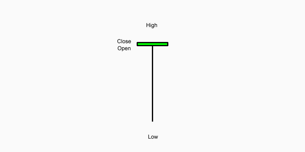
The Inverted Hammer has the following characteristics:
- Small Real Body: The real body (the distance between the open and close prices) is small, which shows that the price did not move much during the trading session. The body can be either at the top or the bottom of the candlestick.
- Long Upper Shadow: The key feature of the Inverted Hammer is its long upper shadow (or wick). This represents a sharp price movement to the upside that was not sustained, signaling that buyers pushed the price higher during the session but were ultimately overpowered by sellers who drove the price back down.
- Little or No Lower Shadow: Ideally, there is little or no lower shadow, although a tiny lower wick is permissible. This suggests that there was little price action on the downside during the session.
- Close Near the Low: The close should be relatively close to the open, and ideally near the bottom of the candlestick, to show that the sellers managed to regain control by the end of the trading period.
Interpretation of the Inverted Hammer
- Location is Key: The Inverted Hammer pattern is most significant when it appears at the bottom of a downtrend. It signals a potential reversal, indicating that despite the prevailing downward trend, the buyers are starting to assert themselves, and a change in direction may be coming.
- Bullish Reversal Signal: The Inverted Hammer suggests that during the trading session, buyers pushed the price higher (long upper shadow), but sellers regained control, causing the price to close near the open. Despite this, the long upper shadow shows that the buying pressure is present and could be an indication that the market is preparing for a bullish reversal.
How to Trade the Inverted Hammer
- Confirmation: The Inverted Hammer alone does not guarantee a reversal. Traders typically look for confirmation in the form of a bullish candlestick that follows it (such as a strong white or green candle) to validate that the market is truly reversing.
- Volume: Higher volume during the formation of the Inverted Hammer increases its reliability. If the price action of the hammer is accompanied by rising volume, it indicates stronger conviction in the market reversal.
- Stop-Loss and Targets: Traders often place a stop-loss just below the low of the Inverted Hammer pattern, in case the reversal does not materialize. The target for this pattern would often be the next significant resistance level or a certain percentage gain from the entry point.
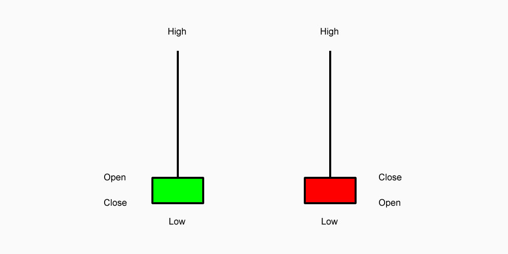
Inverted Hammer vs. Shooting Star
The Inverted Hammer looks similar to the Shooting Star candlestick, but the key difference is their location:
- Inverted Hammer appears in a downtrend and signals a potential reversal to the upside.
- Shooting Star appears in an uptrend and signals a potential reversal to the downside.
While they share a similar structure, their implications differ based on the prevailing market trend.
Example
Imagine a stock that has been in a downtrend for several weeks. On one particular day, the price opens at $50, moves up to $55, and then closes back at $50. The candle formed would have a small body near the bottom of the candle and a long upper shadow, creating an Inverted Hammer. This suggests that buyers tried to push the price higher, but sellers regained control. If the next day shows a strong bullish candlestick, traders may interpret this as a signal to go long, anticipating the start of an upward trend.
Limitations
- False Signals: As with all candlestick patterns, the Inverted Hammer is not foolproof. It can give false signals, especially if there’s no confirmation candle or if it occurs in a strong downtrend without any clear sign of reversal.
- Context Matters: The pattern is more reliable when combined with other technical indicators, such as RSI (Relative Strength Index), moving averages, or support and resistance levels, rather than relying solely on the candlestick pattern.
Conclusion
The Inverted Hammer is a useful candlestick pattern that signals potential bullish reversal when it appears at the bottom of a downtrend. It highlights a shift in market sentiment, where buyers begin to show strength despite the prevailing bearish trend. However, for increased reliability, the pattern should be followed by a confirmation of upward movement, and traders should always consider the broader context and other indicators.