A Cash-Secured Call (also known as a Cash-Backed Call) is a conservative options trading strategy that involves selling a covered call while having sufficient cash or liquid assets set aside to buy the underlying asset if the call is exercised. It’s similar to a covered call but instead of owning the underlying asset, the trader sets aside cash as collateral in case they need to buy the asset.
This strategy is typically used when the investor has a neutral to slightly bullish outlook on the underlying asset and aims to generate income from the premium received by selling the call option. The main difference between a cash-secured call and a standard covered call is that the cash-secured call does not require the investor to already own the underlying asset but instead uses cash to guarantee the potential purchase of the asset.
The objective of a cash-secured call is to generate income through the premiums received from selling the call option while maintaining the ability to purchase the underlying asset if the call is exercised. It’s a neutral to slightly bullish strategy that allows an investor to earn money in a relatively flat or mildly rising market, without having to own the underlying asset in advance.
Maximum Profit
The maximum profit in a cash-secured call strategy is limited to the premium received from selling the call option. Even if the price of the underlying asset rises significantly, the maximum profit is capped at the strike price plus the premium received.
Mathematically:
Maximum Loss
The maximum loss occurs if the price of the underlying asset falls to zero. This is because the trader still holds the cash-secured position but has no offsetting premium income (if the option expires worthless and the asset becomes worthless).
However, because the trader has set aside the cash to buy the asset, the maximum loss is limited to the full price of purchasing the underlying asset at the strike price (which would occur if the call is exercised).
Mathematically:
Breakeven Point
The breakeven point is the price at which the investor will not make a profit or loss from the strategy. It is calculated by taking the strike price of the call and subtracting the premium received from selling the call option.
Mathematically:
Example
Let’s assume a stock is currently trading at $50, and you want to sell a cash-secured call on this stock:
Outcomes
Risk/Reward Profile
Pros
Cons
Example Summary
Aside Cash: $5,500 to buy the stock if exercised
A cash-secured call is a conservative options strategy that generates income through the premiums received from selling call options while setting aside cash to cover the potential purchase of the underlying asset if the option is exercised. It is best used in a neutral to slightly bullish market, where the investor expects little movement or slight appreciation in the asset’s price. The strategy offers limited risk, as the cash set aside can be used to purchase the asset if necessary, but the profit potential is capped at the premium received.
Buying Index Puts is a straightforward and popular options trading strategy used by investors who have a bearish outlook on an underlying stock index. In this strategy, the investor buys a put option on an index (such as the S&P 500, Nasdaq-100, or other indices), which gives the buyer the right, but not the obligation, to sell the underlying index at a specific strike price before or on the expiration date of the option.
The primary goal of buying index puts is to profit from a decline in the value of the underlying index, with the benefit of limited risk. If the index falls significantly below the strike price, the investor can either exercise the put (if the option is in the money) or sell the option to lock in profits.
The objective of buying an index put is to profit from a decline in the value of the underlying index. If the index falls below the strike price of the put option, the option becomes in the money, and the investor can sell the option at a profit or exercise the option to sell the index at a higher price than its current market value.
In simpler terms, buying an index put allows an investor to bet on a decrease in the market or a specific sector represented by the index. If the market falls, the value of the put option increases, potentially resulting in profits.
Maximum Profit
Mathematically:
Maximum Loss
Mathematically:
Breakeven Point
The breakeven point is the index level at which the gains from the put option exactly offset the premium paid. It occurs when the value of the index is equal to the strike price minus the premium paid.
Mathematically:
Example
Let’s say the S&P 500 is currently trading at 4,000, and you expect the index to decline in the next month. Here’s how you might execute a buying index put strategy:
Outcomes
Risk/Reward Profile
When to Buy
Pros
Cons
Example Summary
Buying index puts is a bearish options strategy used to profit from a decline in the value of an underlying index. It offers limited risk (the premium paid) and the potential for unlimited profit if the index falls significantly. This strategy is useful for speculating on market declines, hedging existing positions, or capitalizing on market volatility. However, the strategy requires careful timing, as the option’s value erodes over time, and the investor must anticipate a significant move before expiration to realize a profit.
Buying Index Calls is a straightforward and popular options trading strategy where an investor purchases a call option on an index (such as the S&P 500, Nasdaq-100, or any other financial index). A call option gives the buyer the right, but not the obligation, to buy the underlying asset (in this case, the index) at a specific strike price before or on the expiration date.
When buying an index call, the investor expects that the value of the underlying index will increase (rise) during the life of the option. The primary goal is to profit from price appreciation of the index while limiting the amount of capital at risk (since the risk is limited to the premium paid for the call option).
The main goal of buying index calls is to profit from a rise in the value of the index. If the value of the index increases significantly above the strike price, the investor can exercise the option (if the call option is in the money), or they can sell the option for a profit.
Unlike buying individual stocks, buying options on an index allows the investor to speculate on the overall direction of the market or a broad sector rather than a specific stock.
Maximum Profit
Mathematically:
Maximum Loss
Mathematically:
Breakeven Point
The breakeven point is the price level that the index needs to reach for the buyer to recoup the cost of the premium paid for the option. It is calculated by adding the premium paid for the call to the strike price of the option.
Mathematically:
Example
Let’s say you are interested in the S&P 500 Index (SPX), which is currently trading at 4,000. You believe that the S&P 500 will rise in the coming months. Here’s how you would buy an index call:
Outcomes
Risk/Reward Profile
Pros
Cons
Example Summary
Buying index calls is a bullish strategy that allows investors to profit from an expected rise in the value of an index. The strategy provides limited risk (the premium paid) and unlimited profit potential if the index rises above the strike price. It’s an effective tool for leveraging bullish market views, but the trade must be executed with careful attention to timing, volatility, and the overall market outlook to be successful.
The Bull Put Spread (also known as a Credit Put Spread) is an options trading strategy that is typically used when an investor has a moderately bullish outlook on an underlying asset. The strategy involves selling a put option at a higher strike price and buying a put option at a lower strike price, both with the same expiration date. This setup results in a net credit to the trader’s account, as the premium received from selling the higher strike put is greater than the premium paid for buying the lower strike put.
The Bull Put Spread is a limited-risk, limited-reward strategy that benefits when the price of the underlying asset stays above the strike price of the put option sold (the higher strike) and the options expire worthless.
The goal of a Bull Put Spread is to profit from a stable or moderately bullish move in the underlying asset’s price. The strategy profits when the price of the asset remains above the higher strike price of the sold put option, allowing both puts to expire worthless and the trader to keep the net premium received as profit.
This strategy is designed to limit risk (because the purchased put provides protection) while providing a defined, capped profit potential.
The combination of these two options results in a net credit, meaning the trader receives more money from selling the higher strike put than they pay for buying the lower strike put.
Maximum Profit
Mathematically
Maximum Loss
Mathematically
Breakeven Point
The breakeven point occurs when the price of the underlying asset is such that the profit from the premium received from the short put is exactly offset by the loss on the long put. It is calculated as the strike price of the sold put minus the net premium received.
Mathematically
Example
Let’s say a stock is currently trading at $100. The trader is moderately bullish and wants to create a Bull Put Spread:
Net Premium Received
Maximum Profit
The maximum profit occurs if the stock price remains above $95 at expiration (both options expire worthless).
Maximum Loss
The maximum loss occurs if the stock price falls below $90 at expiration.
Breakeven Point
The breakeven point occurs when the stock price is equal to the strike price of the sold put minus the net premium received.
Risk/Reward Profile
The reward-to-risk ratio can vary depending on the size of the premium received relative to the distance between the two strike prices.
Pros
Cons
Example Summary
The Bull Put Spread (or Credit Put Spread) is a limited-risk, limited-reward strategy used when a trader has a moderately bullish outlook on an underlying asset. It involves selling a higher strike put option and buying a lower strike put option, both with the same expiration date. The strategy benefits from a stable or rising market, with the potential to earn a net premium if the stock price stays above the strike price of the sold put. While the profit is capped, the strategy provides a defined risk and is an efficient way to generate income in moderately bullish market conditions.
The Bull Call Spread (also known as a Debit Call Spread) is a popular options trading strategy used when an investor has a bullish outlook on an underlying asset but wants to limit both the cost and the risk of the trade. The strategy involves buying a call option at a lower strike price and selling a call option at a higher strike price, both with the same expiration date.
This strategy is called a “debit spread” because the trader pays a net debit to enter the position, meaning the cost of buying the call option is higher than the premium received from selling the other call.
The main goal of a Bull Call Spread is to profit from a moderate increase in the price of the underlying asset while limiting both the cost of the trade and the risk. This is done by combining the purchase of a call (which gives unlimited upside potential) with the sale of a call (which offsets part of the cost of the trade, limiting risk).
Mechanics of the Trade
The key feature of the Bull Call Spread is that it allows you to capitalize on a moderate upward movement in the underlying asset’s price, but with limited risk.
Maximum Profit
Mathematically
Maximum Loss
Mathematically
Breakeven Point
The breakeven point occurs when the price of the underlying asset is such that the gains from the long call (the bought call) offset the cost of the trade (the net premium paid). This is calculated as the strike price of the long call plus the net premium paid.
Mathematically
Example
Let’s assume a stock is currently trading at $100. The trader expects the stock to rise moderately but wants to limit their risk.
Net Premium Paid
Maximum Profit
The maximum profit occurs if the stock price is at or above $110 at expiration.
Maximum Loss
The maximum loss occurs if the stock price is below $100 at expiration, as both options would expire worthless.
Breakeven Point
The breakeven point occurs when the stock price is equal to the strike price of the long call plus the net premium paid.
Risk/Reward Profile
When to Use
Pros
Cons
Example Summary
The Bull Call Spread (or Debit Call Spread) is a cost-effective, limited-risk options strategy for traders who are moderately bullish on an asset. It allows the trader to profit from a moderate upward move in the price of the underlying asset while controlling the potential loss. While the profit potential is capped, the strategy provides a balanced risk/reward profile and is well-suited for situations where you expect the underlying asset to rise, but not too dramatically.
The Bear Spread Spread, also known as a Double Bear Spread or Combination Bear Spread, is a sophisticated options strategy that combines elements of two Bear Spread strategies (typically a Bear Put Spread or Bear Call Spread) to create a position with multiple layers of risk and reward. While it’s not as commonly discussed as simpler spreads, it can be an effective tool in specific market conditions.
The goal of the Bear Spread Spread is to create a complex bearish position where the trader can take advantage of the moderate bearish movement of the underlying asset, while limiting risk exposure. This strategy is designed to allow the trader to capitalize on multiple levels of price movement, making it more flexible and potentially more profitable in a market with moderate volatility.
The strategy has limited profit potential but offers greater flexibility in structuring risk-reward scenarios, particularly if a trader believes the underlying asset will decline in stages or at varying rates over time.
Let’s break down a Double Bear Put Spread example:
Example Setup
Imagine you have a stock trading at $100. You are bearish on the stock and want to create a Double Bear Put Spread:
Net Premium Paid
Maximum Profit
Maximum Loss
Breakeven Points
Risk/Reward Profile
Pros
Cons
Example Summary
The Bear Spread Spread (or Double Bear Spread) is a more advanced options strategy that combines two separate Bear Spreads. It’s designed for a moderately bearish outlook and allows for more specific structuring of risk and reward. While the profit potential is capped, it provides flexibility in terms of managing risk over multiple time frames and price ranges. It is most useful in markets where you expect the price of the underlying asset to decline gradually and moderately over time.
A Bear Put Spread is an options trading strategy used when an investor has a bearish outlook on the underlying asset, but wants to limit both the risk and the cost of the trade. It involves buying a put option at a higher strike price and simultaneously selling a put option at a lower strike price, both with the same expiration date.
The strategy benefits from a decline in the underlying asset’s price. The idea is that the price will fall enough for the purchased (long) put to gain value, while the sold (short) put will lose value, but the net loss is limited by the premium collected from the sale.
The goal of a Bear Put Spread is to profit from a decrease in the price of the underlying asset while limiting both the potential loss and the cost of entering the trade. This strategy is typically used when an investor expects the price of the asset to drop but does not anticipate a large move downward.
Maximum Profit
Maximum Loss
Breakeven Point
The breakeven point is the price at which the total value of the position is zero, meaning the profit from the long put is exactly offset by the loss on the short put. The breakeven point is calculated as the higher strike price minus the net premium paid.
Mathematically
Example
Let’s consider an example using a stock currently trading at $100.
Net Premium Paid
Maximum Profit
The maximum profit occurs if the stock price falls below $95 at expiration.
Maximum Loss
The maximum loss occurs if the stock price is above $100 at expiration.
Breakeven Point
The breakeven point is the strike price of the long put minus the net premium paid.
Risk/Reward Profile
Pros
Cons
Example Summary
The Bear Put Spread is a strategy that is ideal for bearish traders who want to limit their risk exposure while still profiting from a moderate drop in the underlying asset’s price. It is a more affordable alternative to simply buying a put option, and its risk and reward are both defined and manageable. However, its profit potential is capped, and it requires the price to decline moderately for maximum profitability.
A Bear Call Spread (also known as a Credit Call Spread) is an options trading strategy used when an investor has a neutral to bearish outlook on the underlying asset. This strategy involves selling a call option at a lower strike price and simultaneously buying a call option at a higher strike price, both with the same expiration date.
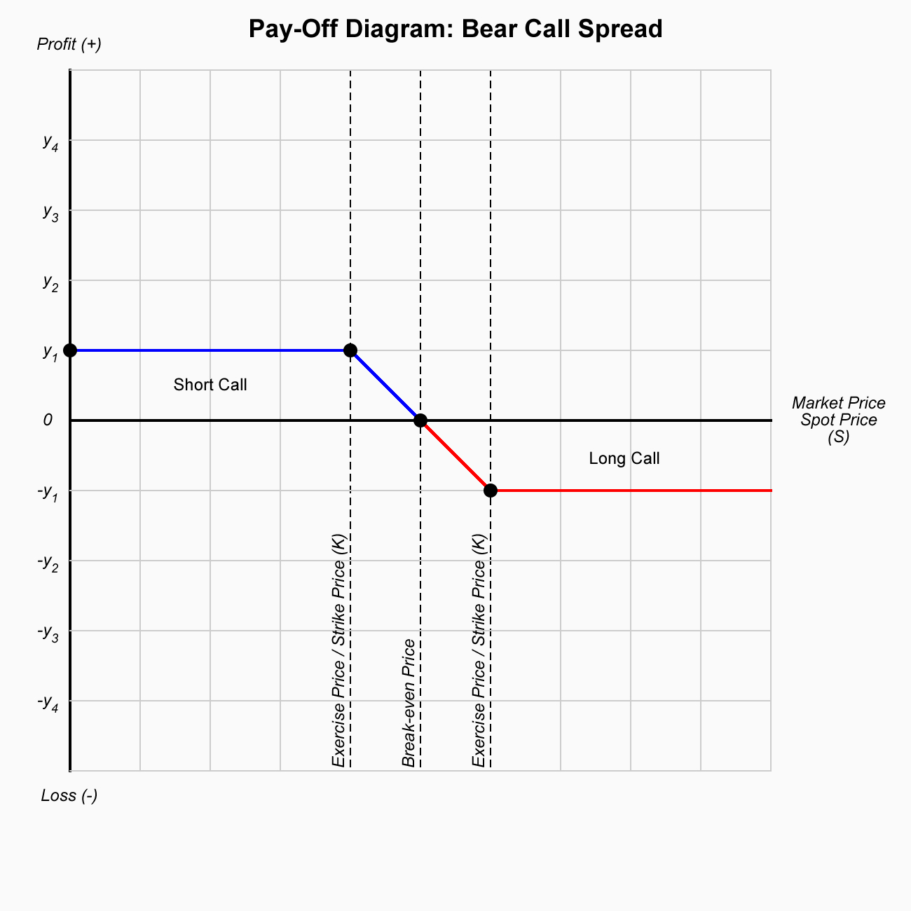
The primary goal of the bear call spread is to generate income through the premium collected from selling the lower strike call option while limiting risk by purchasing the higher strike call option.
Since the strategy is ‘bearish’, it is profitable when the price of the underlying asset remains below the strike price of the call option that was sold (the lower strike), ideally staying as low as possible.
Maximum Profit
Maximum Loss
Breakeven Point
The breakeven point for the trade is calculated by adding the net premium received to the strike price of the short call. Mathematically:
Example
Let’s consider an example using a stock trading at $100:
Net Premium Received
Maximum Profit
The maximum profit occurs if the stock stays below $105 at expiration.
Maximum Loss
The maximum loss occurs if the stock rises above $110 at expiration.
Breakeven Point
The breakeven point is the strike price of the short call plus the net premium received.
Risk/Reward Profile:
Usage
Pros
Cons
The Bear Call Spread is a popular options strategy for those with a neutral to slightly bearish outlook, as it allows traders to collect premium income while limiting downside risk. However, its profit potential is capped, and it requires careful management to avoid significant losses if the price of the underlying asset increases significantly.
In options trading, “the Greeks” refer to a set of risk measures that help traders understand how the price of an option changes in response to various factors. Each Greek measures a specific aspect of an option’s risk profile. Here’s an explanation of the main Greeks:
1. Delta (Δ)
Definition: Delta measures how much the price of an option changes for a $1 change in the underlying asset’s price.
Interpretation:
For call options, delta is positive (0 to 1), meaning the option price will increase as the underlying asset price increases.
For put options, delta is negative (0 to -1), meaning the option price will decrease as the underlying asset price increases.
Example: If a call option has a delta of 0.6, and the underlying stock price rises by $1, the option’s price would increase by $0.60.
The formula for Delta (Δ) in options can be derived from the Black-Scholes model for pricing European-style options. While there are more complex formulas for various options and strategies, the basic formula for Delta in the Black-Scholes framework for a call option and a put option is as follows:
1. Formula for Delta of a Call Option (Δₖ):
Δ
call
=
𝑁
(
𝑑
1
)
2. Formula for Delta of a Put Option (Δₚ):
Δ
put
=
𝑁
(
𝑑
1
)
−
1
Where:
𝑁
(
𝑑
1
)
is the cumulative distribution function (CDF) of the standard normal distribution applied to
𝑑
1
, which represents the probability that the option will end up in-the-money.
𝑑
1
is calculated as:
𝑑
1
=
ln
(
𝑆
𝐾
)
+
(
𝑟
+
𝜎
2
2
)
𝑇
𝜎
𝑇
Where:
𝑆
= Current price of the underlying asset
𝐾
= Strike price of the option
𝑟
= Risk-free interest rate (annualized)
𝜎
= Volatility of the underlying asset (annualized standard deviation)
𝑇
= Time to expiration (in years)
ln
= Natural logarithm
Explanation of the Terms:
𝑁
(
𝑑
1
)
: The cumulative standard normal distribution of
𝑑
1
, which gives the probability of the option expiring in-the-money, adjusted for the current price of the asset, strike price, time to expiration, and volatility.
Δ
call
: For a call option, delta is positive and typically ranges from 0 to 1. It represents the change in the option’s price for a $1 change in the price of the underlying asset.
Δ
put
: For a put option, delta is negative and ranges from 0 to -1. It represents the change in the price of the put option as the underlying asset’s price moves.
Example for a Call Option:
If a call option has a delta of 0.6, it means that for every $1 increase in the underlying asset’s price, the price of the call option will increase by $0.60. Similarly, for a put option, a delta of -0.4 means the price of the put will decrease by $0.40 for every $1 increase in the underlying asset’s price.
Conclusion:
Delta is a measure of an option’s price sensitivity to changes in the price of the underlying asset, and it plays a crucial role in assessing and managing risk in options trading.
2. Gamma (Γ)
Definition: Gamma measures the rate of change of delta in response to changes in the price of the underlying asset. In other words, it shows how delta will change as the price of the underlying asset moves.
Interpretation: Gamma is useful for understanding how much delta might change as the stock price fluctuates. High gamma means delta is more sensitive to price changes.
Example: If a call option has a gamma of 0.05, and the price of the underlying stock increases by $1, the option’s delta will increase by 0.05.
The formula for Gamma (Γ) in options, which measures the rate of change of Delta with respect to changes in the price of the underlying asset, is also derived from the Black-Scholes model for European-style options.
Gamma Formula:
Γ
=
𝑁
′
(
𝑑
1
)
𝑆
𝜎
𝑇
Where:
𝑁
′
(
𝑑
1
)
is the probability density function (PDF) of the standard normal distribution evaluated at
𝑑
1
. This represents the slope of the cumulative distribution function (CDF) at
𝑑
1
.
𝑆
is the current price of the underlying asset.
𝜎
is the volatility of the underlying asset (annualized standard deviation).
𝑇
is the time to expiration (in years).
𝑑
1
is calculated as:
𝑑
1
=
ln
(
𝑆
𝐾
)
+
(
𝑟
+
𝜎
2
2
)
𝑇
𝜎
𝑇
Where:
𝐾
is the strike price of the option.
𝑟
is the risk-free interest rate (annualized).
ln
is the natural logarithm.
Explanation of the Terms:
𝑁
′
(
𝑑
1
)
: This is the PDF of the standard normal distribution. It gives the probability of the underlying asset price being at a certain level (in terms of its normal distribution curve).
Γ
: Gamma represents how much Delta will change when the price of the underlying asset changes. It gives the curvature of the option’s price with respect to the underlying asset’s price. Gamma is always positive for long positions and negative for short positions.
Interpretation:
Gamma is highest when the option is at the money (ATM) and decreases as the option moves further in the money (ITM) or out of the money (OTM).
Gamma tells you how stable Delta is. A higher Gamma means that Delta is more sensitive to changes in the underlying asset’s price.
Example:
If a call option has a Gamma of 0.05, it means that for every $1 increase in the underlying asset’s price, the Delta of the call option will increase by 0.05.
Conclusion:
Gamma helps traders understand how much Delta will change with price movements of the underlying asset, which is crucial for options trading strategies, especially when managing risk. It is used to predict the likelihood of changes in Delta, which is important for hedging and adjusting positions.
3. Theta (Θ)
Definition: Theta measures the rate at which the price of an option decreases as time passes, known as time decay. The closer an option is to its expiration date, the faster its time value erodes.
Interpretation: Options lose value over time, and theta quantifies this loss. Theta is usually negative for both call and put options because, as time passes, the likelihood of an option expiring in the money decreases.
Example: If an option has a theta of -0.05, it will lose $0.05 in value for each day that passes, all else being equal.
The formula for Theta (Θ) in options, which measures the rate of change of an option’s price with respect to the passage of time (i.e., time decay), is derived from the Black-Scholes model for European-style options.
Theta Formula for a Call Option (Θₖ):
Θ
call
=
−
𝑆
⋅
𝑁
′
(
𝑑
1
)
⋅
𝜎
2
𝑇
−
𝑟
⋅
𝐾
⋅
𝑒
−
𝑟
𝑇
⋅
𝑁
(
𝑑
2
)
Theta Formula for a Put Option (Θₚ):
Θ
put
=
−
𝑆
⋅
𝑁
′
(
𝑑
1
)
⋅
𝜎
2
𝑇
+
𝑟
⋅
𝐾
⋅
𝑒
−
𝑟
𝑇
⋅
𝑁
(
−
𝑑
2
)
Where:
𝑆
= Current price of the underlying asset
𝐾
= Strike price of the option
𝑟
= Risk-free interest rate (annualized)
𝜎
= Volatility of the underlying asset (annualized standard deviation)
𝑇
= Time to expiration (in years)
ln
= Natural logarithm
𝑁
(
𝑑
1
)
and
𝑁
(
𝑑
2
)
are the cumulative distribution functions (CDF) for the standard normal distribution, evaluated at
𝑑
1
and
𝑑
2
, respectively.
𝑁
′
(
𝑑
1
)
is the probability density function (PDF) of the standard normal distribution evaluated at
𝑑
1
.
The
𝑑
1
and
𝑑
2
Terms:
𝑑
1
is calculated as:
𝑑
1
=
ln
(
𝑆
𝐾
)
+
(
𝑟
+
𝜎
2
2
)
𝑇
𝜎
𝑇
𝑑
2
is calculated as:
𝑑
2
=
𝑑
1
−
𝜎
𝑇
Explanation of the Formula:
𝑁
′
(
𝑑
1
)
: The PDF of the standard normal distribution at
𝑑
1
. This represents the likelihood of the underlying asset’s price being at a specific level, adjusted for volatility.
𝑒
−
𝑟
𝑇
: The discount factor, accounting for the present value of money, as future cash flows are worth less today.
Time Decay (Theta): Theta is always negative for both call and put options because options lose value as time passes (all else being equal), due to the decreasing probability of the option ending in the money as expiration approaches.
Interpretation:
Theta is typically larger for at-the-money (ATM) options and decreases for in-the-money (ITM) and out-of-the-money (OTM) options as expiration approaches.
Theta tells you how much value an option will lose each day as time decays. For example, if an option has a Theta of -0.05, it means that the option will lose $0.05 in value per day as time passes (assuming other factors remain constant).
Example:
Suppose a call option has a Theta of -0.10, it means that for every day that passes, the option’s value will decrease by $0.10, assuming no change in the price of the underlying asset, volatility, or other factors.
Conclusion:
Theta is a crucial measure in options trading, especially for traders who hold options positions over time. It helps in understanding how the option’s price will decay as expiration approaches and how time affects the profitability of the position. Understanding Theta is especially important for strategies such as selling options (e.g., covered calls, writing puts), where time decay can work in the seller’s favor.
4. Vega (V)
Definition: Vega measures the sensitivity of an option’s price to changes in the volatility of the underlying asset. It indicates how much an option’s price will change with a 1% change in implied volatility.
Interpretation: Higher volatility generally increases the value of both call and put options because it increases the likelihood of large price movements. Therefore, options with higher vega will increase in value if volatility rises.
Example: If an option has a vega of 0.10, and implied volatility increases by 1%, the price of the option will increase by $0.10.
The formula for Vega (V) in options, which measures the sensitivity of an option’s price to changes in the volatility of the underlying asset, is derived from the Black-Scholes model for European-style options.
Vega Formula:
𝑉
=
𝑆
⋅
𝑇
⋅
𝑁
′
(
𝑑
1
)
Where:
𝑆
= Current price of the underlying asset
𝑇
= Time to expiration (in years)
𝑁
′
(
𝑑
1
)
= Probability density function (PDF) of the standard normal distribution evaluated at
𝑑
1
, which is the derivative of the cumulative distribution function (CDF) at
𝑑
1
.
𝑑
1
is calculated as:
𝑑
1
=
ln
(
𝑆
𝐾
)
+
(
𝑟
+
𝜎
2
2
)
𝑇
𝜎
𝑇
Where:
𝐾
= Strike price of the option
𝑟
= Risk-free interest rate (annualized)
𝜎
= Volatility of the underlying asset (annualized standard deviation)
Explanation of the Terms:
𝑁
′
(
𝑑
1
)
: This is the probability density function (PDF) of the standard normal distribution at
𝑑
1
, which represents how much the option’s price changes with a change in volatility of the underlying asset.
𝑆
⋅
𝑇
: This part of the formula represents the relationship between the current price of the underlying asset, time to expiration, and the volatility of the asset. Higher volatility and longer time to expiration increase Vega because the likelihood of a significant price move becomes greater.
Volatility and Vega: Vega is positive for both call and put options. When volatility increases, the option price generally increases because there is a greater chance of the option expiring in-the-money.
Interpretation:
Vega tells you how much the price of an option will change for a 1% change in implied volatility of the underlying asset.
Vega is highest for at-the-money (ATM) options and decreases for in-the-money (ITM) and out-of-the-money (OTM) options as expiration approaches.
Example:
If an option has a Vega of 0.10, it means that if the implied volatility increases by 1%, the price of the option will increase by $0.10.
Conclusion:
Vega is an important Greek in options trading, as it helps traders understand how changes in the volatility of the underlying asset affect the price of an option. Traders use Vega to assess how the market’s view on future volatility might impact their options position. A higher Vega value indicates that the option’s price is more sensitive to changes in volatility, which is especially important for strategies like volatility trading or straddles.
5. Rho (ρ)
Definition: Rho measures the sensitivity of an option’s price to changes in interest rates. It indicates how much the price of an option will change with a 1% change in interest rates.
Interpretation: Generally, rising interest rates tend to increase the value of call options (because the cost of carrying the underlying asset increases) and decrease the value of put options.
Example: If a call option has a rho of 0.05, and interest rates increase by 1%, the price of the call option will increase by $0.05.
The formula for Rho (ρ) in options, which measures the sensitivity of an option’s price to changes in interest rates, is derived from the Black-Scholes model for European-style options.
Rho Formula for a Call Option (ρₖ):
𝜌
call
=
𝐾
⋅
𝑇
⋅
𝑒
−
𝑟
𝑇
⋅
𝑁
(
𝑑
2
)
Rho Formula for a Put Option (ρₚ):
𝜌
put
=
−
𝐾
⋅
𝑇
⋅
𝑒
−
𝑟
𝑇
⋅
𝑁
(
−
𝑑
2
)
Where:
𝐾
= Strike price of the option
𝑇
= Time to expiration (in years)
𝑟
= Risk-free interest rate (annualized)
𝑒
−
𝑟
𝑇
= Discount factor, accounting for the present value of money
𝑁
(
𝑑
2
)
and
𝑁
(
−
𝑑
2
)
are the cumulative distribution functions (CDF) for the standard normal distribution evaluated at
𝑑
2
and
−
𝑑
2
, respectively.
𝑑
2
Calculation:
𝑑
2
=
𝑑
1
−
𝜎
𝑇
Where:
𝑑
1
is calculated as:
𝑑
1
=
ln
(
𝑆
𝐾
)
+
(
𝑟
+
𝜎
2
2
)
𝑇
𝜎
𝑇
Where:
𝑆
= Current price of the underlying asset
𝜎
= Volatility of the underlying asset (annualized standard deviation)
Explanation of the Terms:
𝑁
(
𝑑
2
)
and
𝑁
(
−
𝑑
2
)
: These are the cumulative distribution functions (CDF) for the standard normal distribution, evaluated at
𝑑
2
and
−
𝑑
2
. This part of the formula reflects the likelihood of the option expiring in-the-money adjusted for the interest rate.
𝑒
−
𝑟
𝑇
: This is the discount factor that adjusts the strike price for the time value of money. It reflects the fact that future payments are worth less than present ones due to interest rates.
Interpretation:
Rho represents the change in the option price for a 1% change in the risk-free interest rate.
For call options, Rho is positive, meaning as interest rates rise, the value of the call option increases because the present value of the strike price (which is discounted at the risk-free rate) decreases.
For put options, Rho is negative, meaning as interest rates rise, the value of the put option decreases because the present value of the strike price decreases, making it less attractive to hold the option.
Example:
If a call option has a Rho of 0.05, it means that if the risk-free interest rate increases by 1%, the price of the call option will increase by $0.05.
If a put option has a Rho of -0.04, it means that if the risk-free interest rate increases by 1%, the price of the put option will decrease by $0.04.
Conclusion:
Rho helps traders understand how the price of an option is likely to change in response to interest rate fluctuations. It’s especially important for options traders who are considering positions over long periods of time, as changes in interest rates can have a more significant impact on options with longer expiration dates.
Summary
Delta gives you an idea of how an option’s price will change based on the underlying asset’s price movement.
Gamma shows how sensitive delta is to changes in the price of the underlying asset.
Theta measures how much an option’s price will decay over time.
Vega indicates how much an option’s price is affected by changes in volatility.
Rho reflects how changes in interest rates will affect the option price.
Together, these Greeks help traders manage and assess risk in options positions, making them essential tools for both option buyers and sellers.
The Matching Low candlestick pattern is a simple but useful pattern often found in technical analysis, particularly when traders are analyzing price action in financial markets such as stocks, forex, or commodities. It typically appears in a downtrend and can be interpreted as a potential reversal signal or indication of market indecision.
The Matching Low is a two-candle pattern characterized by two consecutive candlesticks that have the same or nearly identical low prices, but the bodies of the candlesticks can be different in size and color. This pattern suggests that the market has reached a support level where the downward momentum is losing strength.
Imagine a stock is in a downtrend, and it drops to a low of $50. It then rallies to $55, but shortly after, it falls again, testing that $50 low. The price fails to break below $50, and the second candlestick also has a low at exactly $50. This could be interpreted as a Matching Low pattern. If the price starts moving upward after the second candle, it could signal a potential reversal and an opportunity to enter a long (buy) position.
By keeping these key points in mind, you can effectively incorporate the Matching Low pattern into your technical analysis toolbox.