Author Archive Admin

Regression


Overview of Excel’s Regression Output:

When you run a regression analysis in Excel (via the Data Analysis Toolpak), it provides you with several key sections of output:

  • Regression Statistics
  • ANOVA (Analysis of Variance) Table
  • Coefficients Table
  • Residuals (optional, if chosen)

Each of these components helps assess how well the regression model fits your data and gives you insights into the relationship between the dependent and independent variables.

Let’s go through each section in detail:


1. Regression Statistics:

The Regression Statistics section summarizes key metrics about the regression model. The most important pieces here include R-squared, Multiple R, and the Standard Error.

Multiple R

  • Definition: This is the correlation coefficient between the dependent and independent variables. It measures the strength and direction of the linear relationship.
  • Interpretation:
    • A value close to 1 indicates a strong positive linear relationship.
    • A value close to -1 indicates a strong negative linear relationship.
    • A value near 0 indicates little or no linear relationship.

R-squared (R²)

  • Definition: This is the proportion of variance in the dependent variable (Y) that is explained by the independent variable(s) (X). In other words, it shows how well the regression model fits the data.
  • Interpretation:
    • R² ranges from 0 to 1:
      • R² = 1 means the model explains 100% of the variation in Y.
      • R² = 0 means the model explains 0% of the variation in Y.
    • A higher R² indicates a better fit, but it doesn’t mean the model is perfect. It’s also important to check the Adjusted R² for a better assessment of model performance, especially when dealing with multiple predictors.

Adjusted R-squared

  • Definition: Adjusted R² modifies the R² value based on the number of predictors and the sample size. It helps prevent overfitting when multiple variables are added to the model.
  • Interpretation: A higher Adjusted R² suggests a model that fits the data well while accounting for the number of predictors. If Adjusted R² is much lower than R², the model might be overfitting.

Standard Error

  • Definition: This is the standard deviation of the residuals (errors). It measures the average distance between the actual data points and the predicted values.
  • Interpretation:
    • A smaller standard error indicates that the model’s predictions are closer to the actual values, meaning the model has a better fit.
    • A larger standard error suggests more variability in the predictions, meaning the model isn’t explaining the data well.

Observations (n)

  • Definition: The number of data points (or observations) used in the regression analysis.
  • Interpretation: More observations generally provide more reliable results and better statistical power for hypothesis testing.

2. ANOVA (Analysis of Variance):

The ANOVA Table assesses the overall significance of the regression model. It breaks down the variation in the dependent variable into components explained by the model and unexplained (error).

Degrees of Freedom (df)

  • Regression df: This represents the number of independent variables (predictors) in your model. For a simple linear regression, this is usually 1. For multiple regression, it would be the number of predictors.
  • Residual df: The degrees of freedom for residuals (error) is calculated as n – k – 1, where n is the number of observations and k is the number of predictors.
  • Total df: This is the total number of data points minus 1.

Sum of Squares (SS)

  • Regression SS: This represents the variation explained by the regression model. It is the difference between the total variation in the data and the unexplained variation (residuals).
  • Residual SS: This represents the unexplained variation or error. It measures how much the data points deviate from the predicted values.
  • Total SS: The total variation in the data, calculated as the sum of the regression and residual SS. It reflects how much the observed values differ from the mean.

Mean Square (MS)

  • Regression MS: Calculated as Regression SS / Regression df. It measures the average variation explained by the regression model.
  • Residual MS: Calculated as Residual SS / Residual df. It measures the average unexplained variation (error).

F-Statistic

  • Definition: The F-statistic tests the overall significance of the regression model. It compares the model’s explained variance to the unexplained variance.
  • Interpretation:
    • A higher F-statistic suggests that the regression model does a good job explaining the variance in the dependent variable.
    • F-statistic > 1 typically means that the model is significant.

Significance F (p-value for F-statistic)

  • Definition: This is the p-value associated with the F-statistic, which tells you whether the overall regression model is statistically significant.
  • Interpretation:
    • A p-value < 0.05 generally indicates that the regression model is statistically significant (i.e., there is evidence to suggest the independent variable has an effect on the dependent variable).
    • A p-value ≥ 0.05 suggests that the model may not be statistically significant, and there may not be a meaningful relationship between the independent and dependent variables.

3. Coefficients Table:

The Coefficients Table shows the values of the regression coefficients, which are the estimated parameters for the regression equation. These coefficients tell you how each independent variable (predictor) influences the dependent variable.

Intercept (Constant)

  • Definition: The intercept is the expected value of the dependent variable when all independent variables are 0.
  • Interpretation: The intercept represents the starting point of the regression line. In many cases, it may not have much practical significance, especially if 0 isn’t within the plausible range of the independent variables.

Coefficients for Independent Variables (X)

  • Definition: The coefficient of each independent variable represents the change in the dependent variable for a 1-unit change in that independent variable, holding all other variables constant.
  • Interpretation:
    • A positive coefficient means that as the independent variable increases, the dependent variable is expected to increase.
    • A negative coefficient means that as the independent variable increases, the dependent variable is expected to decrease.
    • The magnitude of the coefficient tells you the strength of the relationship.

Standard Error of Coefficients

  • Definition: The standard error of each coefficient measures the variability or precision of the coefficient estimate.
  • Interpretation: A smaller standard error suggests the coefficient is estimated more precisely.

t-Statistic

  • Definition: The t-statistic tests whether the coefficient is significantly different from 0. It’s calculated as coefficient / standard error.
  • Interpretation:
    • A larger absolute t-statistic suggests that the coefficient is more likely to be significantly different from 0.
    • The rule of thumb is that if |t-statistic| > 2, the coefficient is considered statistically significant.

P-value for Coefficients

  • Definition: This tests the null hypothesis that the coefficient is equal to zero (i.e., no effect).
  • Interpretation:
    • A p-value < 0.05 means the coefficient is statistically significant (indicating that the predictor variable has a meaningful effect on the dependent variable).
    • A p-value ≥ 0.05 suggests that the coefficient is not significantly different from 0, and the corresponding variable might not be a meaningful predictor of the dependent variable.

Confidence Intervals for Coefficients (Lower 95% and Upper 95%)

  • Definition: The confidence interval gives the range of values within which we can be 95% confident the true coefficient lies.
  • Interpretation: If the confidence interval does not include 0, it supports the idea that the predictor variable is statistically significant.

4. Residuals:

Residuals are the differences between the observed data points and the values predicted by the model. Analyzing residuals helps you evaluate how well the model fits the data.

Residuals (Observed – Predicted)

  • Definition: Residuals are the errors of the regression model, calculated as the difference between the actual values and the predicted values.
  • Interpretation:
    • Ideally, residuals should be randomly scattered around 0, indicating that the model doesn’t systematically underpredict or overpredict the dependent variable.
    • Patterns or trends in residuals might indicate model misspecification or that there’s a non-linear relationship that the linear model cannot capture.

Standardized Residuals

  • Definition: Standardized residuals are scaled versions of the residuals. They help to identify outliers by expressing the residuals in terms of standard deviations.
  • Interpretation:
    • A standardized residual larger than ±2 or ±3 may indicate an outlier, meaning the data point is significantly different from the model’s prediction.

Comprehensive Analysis Summary:
  • Model Significance: The Significance F and p-values for coefficients give you an idea of whether the model as a whole and individual predictors are significant.
  • Goodness of Fit: R-squared, Adjusted R², and F-statistics help you understand how well the model fits the data and whether it explains a meaningful portion of the variance.
  • Variable Impact: The coefficients indicate how each predictor influences the dependent variable. Look at their magnitude and sign (positive or negative) to understand relationships.
  • Model Adequacy: Check residuals to ensure there’s no systematic bias in your model and that it appropriately captures the data.

With all these components, you can thoroughly assess the performance and reliability of your regression model and ensure that it provides meaningful insights.

Greek Alphabet


UppercaseLowercaseName
Ααalpha
Ββbeta
Γγgamma
Δδdelta
Εεepsilon
Ζζzêta
Ηηêta
Θθthêta
Ιιiota
Κκkappa
Λλlambda
Μμmu
Ννnu
Ξξxi
Οοomikron
Ππpi
Ρρrho
Σσ, ςsigma
Ττtau
Υυupsilon
Φφphi
Χχchi
Ψψpsi
Ωωomega

Parameters


ParameterDescription
S0spot price at inception of the contract (t=0)
FPforward price
Rfannual risk-free rate
Tforward contract term (years)

Mark-to-Market (MTM)


What is Mark-to-Market (MTM)?

Mark-to-market is an accounting practice or process that involves adjusting the value of an asset or a liability to reflect its current market value rather than its book value or historical cost. The goal of MTM is to ensure that financial statements reflect the true current value of assets and liabilities as determined by the latest market prices.

In the context of futures contracts, MTM refers to the daily process of revaluing the contract based on the market’s closing price and adjusting the margin accounts of the involved parties accordingly.


The MTM Process in Futures Contracts
  1. Daily Revaluation:
    • Futures contracts are marked-to-market at the end of each trading day based on the closing price of the underlying asset. This means that the contract is revalued to reflect the most up-to-date market conditions, essentially recalculating what the contract is worth at that moment.
    • The contract’s price moves according to the underlying asset’s price fluctuations. If the futures price rises or falls relative to the previous day’s settlement price, the value of the futures contract will change.
  2. Settlement of Gains and Losses:
    • The difference between the closing price of the futures contract at the end of each day and the price at the previous day’s close represents the gain or loss.
    • If the value of the futures contract increases (for the holder of a long position, or a “buyer”), the buyer gains, and the seller loses by the same amount. If the value decreases, the seller gains, and the buyer loses by the same amount.
    • These gains and losses are settled daily, meaning that they are either credited or debited to the margin accounts of the traders. This daily settlement process prevents the accumulation of large losses over time.
  3. Margin Requirements:
    • Initial Margin: This is the amount of money a trader must deposit with the exchange to open a position. It’s a good faith deposit to ensure the trader can fulfill their financial obligations in the contract.
    • Maintenance Margin: This is the minimum balance required in a trader’s margin account to keep a position open. If the balance in the margin account drops below this level due to daily losses, the trader receives a margin call and must deposit additional funds to bring the margin back up to the required level.
    • The initial margin is the amount needed to enter the position, while the maintenance margin is the threshold below which the position will be liquidated if additional funds are not added.
  4. Resetting the Contract’s Value to Zero:
    • The contract’s value is reset to zero at the end of each trading day after gains and losses are settled. This means that traders are not holding on to the profit or loss from the previous day but instead, are working with a fresh starting point for the next day.


Key Features of Mark-to-Market
  • Real-Time Reflection of Market Conditions: MTM ensures that the value of the futures contract is always aligned with the current market value of the underlying asset. This helps to maintain transparency and accuracy in financial reporting, as the value is updated to reflect what the asset is worth at any given moment.
  • Reduces Counterparty Risk: By adjusting the value of contracts daily and settling gains and losses regularly, MTM helps reduce the risk that a counterparty may default on their obligations. The daily settlements mean that traders are always on top of their positions, and their exposure is not allowed to build up over time.
  • Liquidity and Flexibility: The daily settlement of gains and losses also helps keep the futures market liquid and dynamic. Traders can quickly adjust their positions, either adding more margin to cover losses or liquidating their position if the market moves unfavorably.


Why is Mark-to-Market Important?
  • Transparency and Accuracy: MTM allows for a more accurate reflection of a contract’s value, ensuring that financial statements reflect the true economic value of assets and liabilities.
  • Regulatory Compliance: Many financial markets and regulatory bodies require the use of MTM accounting to ensure fairness and to minimize systemic risk, particularly in markets like futures and other derivative contracts.
  • Risk Management: MTM helps manage and limit risk by ensuring that gains and losses are realized and settled daily, allowing traders to take immediate action if necessary, such as depositing additional margin or closing positions.


Mark-to-Market Outside of Futures Contracts

Mark-to-market is not limited to futures markets—it also applies to a range of other financial assets, including:

  • Equities: Stocks can be marked-to-market at the end of each trading day, adjusting their value to reflect the current market price.
  • Bonds: Bond prices can be marked-to-market by considering the yield and price of similar instruments in the market.
  • Derivatives: Options, swaps, and other derivatives are also subject to MTM, which reflects their real-time market value, based on the underlying asset’s current price.


Example of MTM in Action (Futures Contract)

Let’s say a trader enters into a long futures contract on oil with a price of USD 70 per barrel. Here’s how MTM would work:

  • On Day 1, the futures price is USD 70. The trader deposits an initial margin of USD 5,000.
  • On Day 2, the price rises to USD 72 per barrel. The trader’s account is credited with the gain of USD 2 per barrel.
  • On Day 3, the price falls to USD 71. The trader’s account is debited USD 1 per barrel.
  • On Day 4, the price rises again to USD 73. The trader’s account is credited USD 2 per barrel.

Each day, the trader’s margin account is adjusted according to the daily change in the contract’s value, ensuring that the position is fully collateralized and reflecting the real-time market value of the contract.


Conclusion

Mark-to-market is an essential process for ensuring that the values of financial contracts, particularly in futures markets, are accurately and transparently reflected based on current market conditions. It helps to manage risk, ensure liquidity, and provide up-to-date financial reporting, all while preventing large-scale losses or defaults. The MTM system of daily settlement and revaluation promotes efficiency and stability in financial markets.


Risk Premium


A risk premium is the additional return or yield that an investor requires for taking on the extra risk associated with an investment compared to a risk-free alternative. In other words, it compensates investors for bearing uncertainty or potential losses that come with riskier assets.


The formula for the Risk Premium is generally expressed as the difference between the expected return on a risky asset and the return on a risk-free asset. Here’s the formula:


Risk Premium = Expected Return on Risky Asset − Risk-Free Rate


\text{Risk Premium} = \text{Expected Return on Risky Asset} – \text{Risk-Free Rate}

Where:

  • Expected Return on Risky Asset is the return that investors anticipate earning from a specific risky asset (e.g., a stock, corporate bond, or long-term government bond).
  • Risk-Free Rate is the return on an asset considered to be free of risk, often represented by the return on short-term government bonds (such as U.S. Treasury bonds).


Example:

If the expected return on a corporate bond is 6%, and the risk-free rate (say, the return on a 1-year Treasury bond) is 2%, the risk premium would be:


Risk Premium=6%2%=4%\text{Risk Premium} = 6\% – 2\% = 4\%


This means that investors require an additional 4% return for taking on the risk of the corporate bond, as compared to the risk-free Treasury bond.


Additional Forms of Risk Premiums
  • Equity Risk Premium: For stocks, the risk premium is the difference between the expected return on the stock market (or a specific stock) and the risk-free rate.
    Equity Risk Premium=Expected Return on StocksRisk-Free Rate\text{Equity Risk Premium} = \text{Expected Return on Stocks} – \text{Risk-Free Rate} 
  • Credit Risk Premium: For bonds, it’s the difference between the yield on a corporate bond and the yield on a government bond of similar maturity.
    Credit Risk Premium=Yield on Corporate BondYield on Government Bond\text{Credit Risk Premium} = \text{Yield on Corporate Bond} – \text{Yield on Government Bond} 

In these cases, the formula follows the same basic structure but is applied to different assets (stocks, corporate bonds, etc.).


Key Points about Risk Premium
  1. Risk vs. Risk-Free Asset:
    • Risk-free assets are investments that are considered to have no risk of default or loss, such as government bonds from a stable country (e.g., U.S. Treasury bonds).
    • Risky assets include investments like stocks, corporate bonds, or even long-term government bonds from less stable countries, which carry the possibility of higher returns but also greater risk (e.g., market volatility or default risk).

    The difference between the return on a risky asset and the return on a risk-free asset is the risk premium.

  2. Compensation for Risk:
    • The idea is that investors expect higher returns for taking on higher levels of risk. For example, an investor in corporate bonds might demand a higher return than they would receive from a government bond, compensating them for the risk of the corporation defaulting on its debt.
  3. Types of Risk Premiums:
    • Equity Risk Premium: The additional return that investors expect to earn from investing in stocks over the return on risk-free assets (e.g., U.S. Treasury bonds).
    • Credit Risk Premium: The extra yield that investors demand for holding bonds issued by borrowers who are not considered risk-free (i.e., corporate bonds or bonds from countries with weaker credit ratings).
    • Liquidity Premium: Investors may require a premium for holding assets that are not easily tradable or that take longer to sell without affecting the price.
    • Term Premium: The additional return for holding long-term bonds compared to short-term bonds, compensating for interest rate risk (the risk that interest rates will change unfavorably over time).
  4. Why It Exists:
    • Uncertainty: Riskier investments have more uncertainty about future returns. Investors demand compensation for taking on that uncertainty.
    • Volatility: The higher the potential for volatility or loss, the higher the risk premium that investors demand.
    • Default Risk: If there’s a chance that an issuer of debt might not pay back the principal or interest (as with corporate bonds or bonds from riskier countries), investors will require a risk premium.


Example of Risk Premium

Let’s say the risk-free rate (the return on a 1-year U.S. Treasury bond) is 2%, and you’re considering investing in a corporate bond with a higher risk of default. If the expected return on the corporate bond is 5%, the risk premium for this bond would be 5% – 2% = 3%.


How Risk Premiums Affect Financial Markets
  • Investors’ Choices: Investors will compare the risk premiums offered by different investments and choose those that align with their risk tolerance and return expectations.
  • Asset Prices: Risk premiums can affect asset prices. If the perceived risk of an asset increases, the required risk premium will also increase, causing the price of the asset to fall (since higher yields are demanded by investors).
  • Economic Implications: A higher overall risk premium in the market may signal increased uncertainty or risk aversion among investors, which can influence economic conditions and investment decisions.


Risk Premium and the Unbiased Expectation Hypothesis (UEH)

In the context of the Unbiased Expectation Hypothesis, if there were a risk premium in play, long-term interest rates would no longer be an unbiased reflection of future short-term rates. Instead, long-term rates would also incorporate a premium for the risk of holding longer-term securities. This would make the relationship between short-term and long-term rates more complex, as investors would be demanding a premium to compensate for the uncertainty over time.

In summary, the risk premium is a fundamental concept in finance, representing the extra return investors demand to compensate for the risks they assume when investing in assets that are not risk-free.


Present Value (PV)


Discreet Compounding


The formula for the present value with discrete compounding is:


$$PV=\frac{FV}{\left( 1+\frac{r}{n} \right)^{nt}}$$


Where:

  • PV = Present value
  • FV = Future value
  • r = Interest rate (as a decimal)
  • n = Number of compounding periods per year
  • t = Time in years


This formula calculates the present value of a future cash flow, discounted at an interest rate r, with n compounding periods per year, over a period of t years.


Continuous Compounding


The formula for the present value with continuous compounding is:


$$PV=FV⋅e^{−𝑟𝑡}$$

PV = P \cdot e^{-rt}


Where:

  • PV = Present Value
  • FV = Future Value
  • r = interest rate (decimal)
  • t = time (years)
  • e = Euler’s number (approximately 2.71828)


This formula calculates the present value of a future cash flow when interest is compounded continuously at a rate r over time t.


Present Value (Discreet Compounding)


Test!
Test!
Years
Present Value:


The given formula is:

$$F_{0}(T) = S_{0}*(1+r)^T$$


To solve for

TT

, we can follow these steps:

(1) Divide both sides of the equation by

S0S_0

:

$$\frac{F_{0}(T)}{S_{0}} = (1+r)^T$$


(2) Take the natural logarithm (ln) of both sides:

$$ln\left( \frac{F_{0}(T)}{S_{0}} \right) = ln\left( (1+r)^T \right)$$


(3) Use the logarithmic identity

ln(ab)=bln(a)\ln(a^b) = b \ln(a)

:

$$ln\left( \frac{F_{0}(T)}{S_{0}} \right) = T*ln(1+r)$$


Finally, solve for

TT

by dividing both sides by

ln(1+r)\ln(1 + r)

:

$$T=\frac{ln\left( \frac{F_{0}(T)}{S_{0}} \right)}{ln(1+r)}$$


So the formula to find T is:

$$T=\frac{ln\left( \frac{F_{0}(T)}{S_{0}} \right)}{ln(1+r)}$$


xxx

Collar (Protective Collar)


A Collar (also known as a Protective Collar) is a popular options strategy that combines the use of a long position in the underlying asset, a covered call, and a protective put. The purpose of a collar is to limit potential losses on the underlying asset while also capping potential gains. This strategy is often used by investors who want to protect themselves from downside risk, but who are also willing to limit their upside potential in exchange for that protection.


Pay-Off Diagram


Options - Collar (Protective Collar)


Key Elements
  1. Long Position in the Underlying Asset: The investor holds shares (or another asset) that they are concerned about losing value in, but still want to retain some exposure to the asset.
  2. Selling a Covered Call: The investor sells a call option on the asset at a strike price higher than the current market price. This generates income through the premium received from selling the call, which can help finance the cost of buying the protective put. The covered call also caps the potential gains because if the price of the asset rises above the strike price, the investor will be forced to sell the asset at that price.
  3. Buying a Protective Put: The investor buys a put option on the same underlying asset at a strike price lower than the current market price. This put option provides downside protection, ensuring that if the price of the asset falls, the investor can sell the asset at the put’s strike price, thus limiting their potential losses.


Objectives

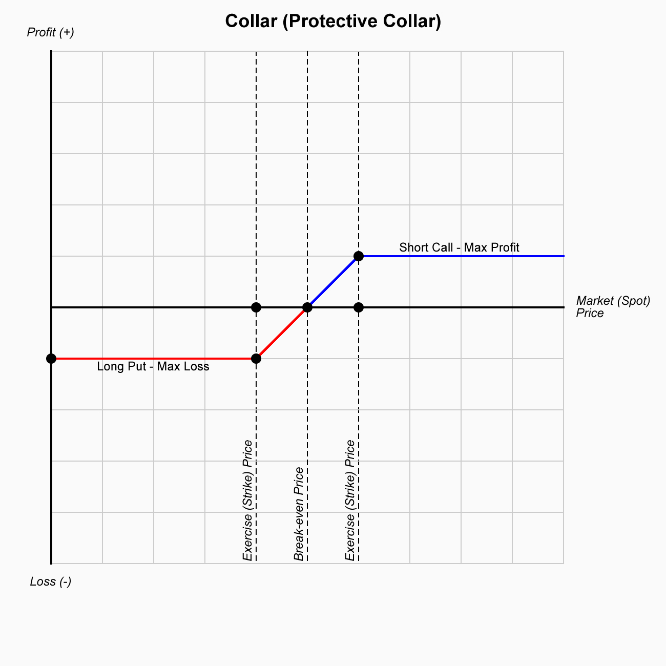
The collar strategy is used to limit downside risk while also capping upside potential. This strategy is suitable for investors who want to protect their gains or limit losses in a volatile or uncertain market but are willing to forgo unlimited potential profits in return for the protection provided by the put option.


Mechanics

The collar strategy typically involves the following steps:

  1. Hold the Underlying Asset: The investor owns shares or an equivalent amount of the underlying asset (e.g., stocks, ETFs, etc.).
  2. Sell a Covered Call: The investor sells a call option with a strike price higher than the current market price of the underlying asset. This allows them to collect a premium upfront, which can help offset the cost of purchasing the protective put.
  3. Buy a Protective Put: The investor buys a put option with a strike price lower than the current market price. This limits the potential loss on the position if the price of the underlying asset falls significantly.

The protective collar limits both potential losses (through the protective put) and potential gains (through the sold call option). The cost of buying the protective put is partially or fully offset by the premium received from selling the call option, making it an affordable risk management strategy for some investors.


Example

Let’s consider an investor who owns 100 shares of a stock currently trading at $50 per share. The investor wants to limit potential losses but also wants to potentially profit from some upside movement. The investor decides to implement a collar strategy by selling a covered call and buying a protective put.

  1. Hold the Underlying Asset: The investor holds 100 shares of the stock at $50 per share.
  2. Sell a Covered Call: The investor sells a call option with a strike price of $55, expiring in one month, for a premium of $2 per share. The total premium received is $200 (since one options contract represents 100 shares).
  3. Buy a Protective Put: The investor buys a put option with a strike price of $45, expiring in one month, for a premium of $1 per share. The total cost of the put option is $100.

In this case, the investor is using the $200 premium from the covered call to help offset the cost of the $100 premium for the protective put. Therefore, the net cost of the collar strategy is $100 ($200 premium from the call minus $100 cost of the put).


Possible Outcomes
  • If the stock price rises above $55:
    • The investor will be obligated to sell the stock at $55 (due to the covered call). The stock is sold at the strike price of the call option.
    • The profit from this scenario is limited to the difference between the initial stock price and the strike price of the call option, plus the premium received.
    • For example, if the stock rises to $60, the investor sells the stock at $55, generating a $5 per share profit, plus the $2 premium from the call. The total profit is $7 per share.
  • If the stock price stays between $45 and $55:
    • The put option expires worthless, and the investor keeps the stock. The call option also expires worthless, so the investor keeps the premium from the call ($200) but has no obligation to sell the stock.
    • In this scenario, the investor’s effective profit is the premium received from selling the call ($200), minus the cost of the put ($100), for a net gain of $100.
  • If the stock price falls below $45:
    • The put option is exercised, and the investor is able to sell the stock at $45 (the strike price of the put option).
    • The maximum loss is limited to the difference between the current stock price and the put strike price, minus the premium received from the call. For example, if the stock falls to $40, the investor will sell it at $45, avoiding further losses below that price. The maximum loss would be $5 per share (from the initial price of $50 to the put strike price of $45), but this is offset by the $2 premium received from the call, so the net loss is $3 per share.


Risk/Reward Profile
  • Maximum Profit: The maximum profit in a collar strategy is limited to the strike price of the sold call (minus the purchase price of the stock) plus the premium received from selling the call. If the price of the underlying asset rises above the call strike price, the investor will be forced to sell the asset at the strike price, and any further price increases are not captured.
    • Example: If the stock rises to $60, the maximum profit is $55 (strike price of the call) minus the $50 purchase price of the stock, plus the $2 premium received from the call, for a total maximum profit of $7 per share.
  • Maximum Loss: The maximum loss occurs if the price of the underlying asset falls below the strike price of the put, but the loss is capped at the difference between the stock’s current price and the put’s strike price (less the premium received from selling the call).
    • Example: If the stock falls to $40, the maximum loss is $50 (purchase price of the stock) minus $45 (put strike price), plus the cost of the put premium ($100). This results in a maximum loss of $300 (or $3 per share), which is a limited loss compared to the potential loss without the collar.
  • Breakeven Point: The breakeven point occurs at the current price of the stock minus the premium received from the call option, plus the cost of the put option.
    • Example: If the stock is at $50, the net premium received from the call is $200, and the cost of the put is $100. The breakeven point is $50 (current stock price) – $2 (call premium) + $1 (put premium) = $49 per share.


Pros
  1. Downside Protection: The protective put provides downside protection, limiting potential losses if the price of the underlying asset falls sharply.
  2. Income Generation: The premium received from selling the call option generates immediate income, which can help offset the cost of the put option or contribute to the overall return.
  3. Defined Risk/Reward: The collar strategy provides a defined risk and defined reward. Investors know the maximum potential loss and gain upfront, which can help with risk management and planning.
  4. Cost-Effective: In many cases, the premium received from selling the covered call can offset the cost of buying the protective put, making this strategy relatively inexpensive for the investor.


Cons
  1. Limited Upside Potential: The collar strategy caps potential profits. If the underlying asset rises significantly above the call’s strike price, the investor will not benefit from the additional price increase. They are obligated to sell the asset at the strike price of the call option.
  2. Opportunity Cost: While the investor has limited downside risk, the strategy also limits the upside potential, which could be frustrating if the underlying asset performs very well.
  3. Complexity: The collar strategy can be more complex than simply holding the underlying asset, as it requires managing multiple options contracts (buying a put and selling a call) while maintaining a long position in the underlying asset.
  4. Transaction Costs: There can be significant transaction costs associated with implementing the collar, especially when buying and selling options contracts frequently.


When to Use
  • Protect Gains: The collar is ideal for investors who have gained a substantial amount of value in an asset and want to lock in profits while still having limited exposure to downside risk.
  • Uncertain Market Conditions: This strategy is well-suited for times when the investor expects volatility in the market but is unsure of the direction. It provides a hedge against large losses while still allowing for some upside potential.
  • Neutral to Moderately Bullish: The investor believes that the asset’s price will stay within a specific range or rise moderately, but they want to limit losses if the price falls.


Conclusion

The collar (protective collar) strategy is a risk management tool that allows investors to protect against downside risk while capping potential upside gain. By combining a long position in the asset, selling a covered call, and buying a protective put, the collar provides a defined risk/reward profile. This strategy is useful for investors looking to hedge their positions in volatile markets, protect gains, or generate income through options premiums, while also being willing to limit potential profits. The strategy works well in markets with uncertainty or volatility and is especially attractive to investors with neutral to slightly bullish outlooks.


Cash-Secured Put


A Cash-Secured Put is an options trading strategy that involves selling a put option while setting aside sufficient cash to purchase the underlying asset (if the put option is exercised). This strategy is commonly used by investors who are willing to buy the underlying asset at a certain price (the strike price of the put) in exchange for receiving an upfront premium from selling the put option.

This strategy is considered conservative and is typically employed when an investor has a neutral to slightly bullish outlook on the underlying asset and is looking to generate income through premiums while potentially acquiring the asset at a price lower than its current market value.


Key Elements
  1. Sell a Put Option: In this strategy, the investor sells a put option on a particular asset (like a stock, ETF, or index). By selling the put, the investor agrees to potentially buy the underlying asset at the strike price if the option is exercised by the buyer.
  2. Set Aside Cash: The key characteristic of a cash-secured put is that the investor sets aside enough cash to purchase the underlying asset at the strike price if the put option is exercised. This ensures the investor can fulfill their obligation if the option is exercised.
  3. Income Generation: By selling the put option, the investor receives a premium, which is the income generated from the strategy. The premium is kept regardless of whether the option is exercised, making this a potentially lucrative strategy when markets are flat or slightly bullish.
  4. Neutral to Slightly Bullish Outlook: The investor typically has a neutral to slightly bullish outlook on the underlying asset. They may want to own the asset but are not willing to buy it at the current market price, so they are willing to potentially buy it at the lower strike price, collecting premium income in the process.


Objective

The main goal of a cash-secured put is to generate income from the premium received from selling the put option while keeping the possibility of acquiring the underlying asset at a discount (the strike price) if the option is exercised. It is used in scenarios where the investor is willing to buy the asset at the strike price but is also content with keeping the premium if the option expires worthless.


Mechanics
  1. Sell a Put Option: The trader sells a put option with a specific strike price and expiration date. This obligates them to buy the underlying asset at the strike price if the put option is exercised by the buyer.
  2. Set Aside Cash: The trader sets aside enough cash to purchase the underlying asset if the put is exercised. For example, if the strike price is $100 per share and the investor sells one put contract (which typically represents 100 shares), they must set aside $10,000 in cash to cover the purchase of 100 shares at the strike price.
  3. Receive Premium: The trader receives the premium from selling the put option. This premium is theirs to keep, regardless of whether the option is exercised or expires worthless.
  4. Expiration or Exercise:
    • If the underlying asset price stays above the strike price: The put option expires worthless, and the investor keeps the premium as profit without having to buy the underlying asset.
    • If the underlying asset price falls below the strike price: The put option is exercised, and the trader is obligated to buy the underlying asset at the strike price. In this case, the premium received from selling the put option helps to reduce the effective cost of acquiring the asset.


Maximum Profit

The maximum profit occurs when the put option expires worthless (i.e., the price of the underlying asset remains above the strike price). In this case, the investor keeps the full premium received for selling the put option as profit.


Mathematically:

  • Maximum Profit = Premium Received.


Maximum Loss

The maximum loss occurs if the price of the underlying asset falls to zero. In this case, the investor would have to buy the asset at the strike price, which would result in a significant loss. However, this loss is partially offset by the premium received from selling the put option.


Mathematically:

  • Maximum Loss = Strike Price of the Put – Premium Received (if the asset price falls to zero).


Breakeven Point

The breakeven point is the price at which the investor will neither make a profit nor a loss. It occurs when the price of the underlying asset is equal to the strike price minus the premium received.


Mathematically:

  • Breakeven = Strike Price – Premium Received.


Example

Let’s say an investor is interested in selling a cash-secured put on a stock currently trading at $50. The investor decides to sell a put option with a strike price of $45, expiring in one month, and receives a premium of $2 per share.

  1. Sell the Put Option: The investor sells a put option with a strike price of $45, expiring in one month, for a premium of $2 per share.
  2. Set Aside Cash: Since the strike price is $45, the investor must set aside enough cash to buy the stock at that price if the option is exercised. For one options contract (100 shares), this amounts to $4,500.
  3. Premium Received: The investor collects $2 per share, or $200 (100 shares x $2).


Outcomes

  • If the stock stays above $45:
    • The put option expires worthless, and the investor keeps the $200 premium as profit. The investor does not need to buy the stock.
  • If the stock falls to $40:
    • The put option is exercised, and the investor is obligated to buy the stock at $45.
    • The investor spends $4,500 to buy 100 shares of the stock at $45 each.
    • The effective cost of the stock is reduced by the $200 premium, so the effective cost is $4,300 ($4,500 – $200 premium received).
    • The investor now owns the stock at an average cost of $43 per share, even though the market price is $40 per share.
  • If the stock falls to $0:
    • The investor is still obligated to buy the stock at $45, but now the stock is worth nothing.
    • The loss is $4,500 (the total amount spent to buy the stock) minus the $200 premium received, resulting in a net loss of $4,300.


Risk/Reward Profile
  • Maximum Loss: The maximum loss occurs if the price of the underlying asset falls to zero, in which case the investor would incur a loss equal to the strike price minus the premium received. However, the loss is mitigated by the premium income.
    • Maximum Loss = Strike Price – Premium Received (if the asset’s value drops to zero).
  • Maximum Profit: The maximum profit is limited to the premium received for selling the put option. The investor cannot earn more than the premium, even if the underlying asset’s price rises significantly.
    • Maximum Profit = Premium Received.
  • Breakeven Point: The breakeven point is the price at which the net result of the strategy is zero, accounting for both the premium received and the price of the underlying asset.
    • Breakeven = Strike Price – Premium Received.


When to Use
  1. Neutral to Bullish Outlook: The investor expects the price of the underlying asset to either stay the same or increase slightly, but they are willing to buy the asset at the strike price if the market falls.
  2. Generate Income: This strategy is ideal for generating income through premiums in a relatively stable or slightly bullish market. If the market remains above the strike price, the premium is a profitable outcome for the trader.
  3. Willing to Acquire the Asset: This strategy is best suited for investors who are willing to own the underlying asset at a price lower than the current market price. The investor may view the potential acquisition as an opportunity to purchase the asset at a discounted price if the market price falls.


Pros

  1. Income Generation: The premium received from selling the put option provides immediate income to the investor, which can be especially attractive in flat or slightly bullish markets.
  2. Limited Risk: The risk is limited to the difference between the strike price and the premium received if the asset falls to zero. This makes it a relatively low-risk strategy when compared to strategies like selling naked puts or shorting the asset outright.
  3. Potential Discounted Purchase: If the option is exercised, the investor can acquire the underlying asset at a discounted price (the strike price minus the premium).
  4. Ideal for Neutral or Slightly Bullish Markets: This strategy works best when the investor believes the price of the asset will not fall below the strike price.


Cons

  1. Limited Profit Potential: The maximum profit is capped at the premium received, so even if the underlying asset rises significantly, the investor will only profit from the premium.
  2. Cash Requirement: The strategy requires the investor to set aside a significant amount of cash (equal to the strike price of the put multiplied by 100 shares per contract), which can tie up capital and reduce liquidity.
  3. Risk of Ownership: If the price of the underlying asset falls below the strike price, the investor will have to buy the asset, and the value of that asset may continue to decline, leading to potential losses.
  4. Missed Opportunity: If the market price stays above the strike price, the investor misses the opportunity to purchase the asset at a lower price, especially if the price drops after the option expires.


Example Summary

  • Stock Price: $50
  • Sell Put Option with Strike Price of $45
  • Premium Received: $2 per share
  • Set Aside Cash: $4,500 (for 100 shares)
  • Maximum Profit: $200 (premium received)
  • Maximum Loss: $4,300 (if the stock falls to zero)
  • Breakeven: $43 (strike price – premium received)


Conclusion

A cash-secured put is a relatively conservative strategy used to generate income through the premium received from selling put options, while also providing the opportunity to acquire the underlying asset at a discount if the option is exercised. The strategy is best suited for investors with a neutral to bullish outlook who are willing to own the asset at the strike price and are looking to generate income in a stable or slightly bullish market. The maximum risk is limited to the strike price of the put minus the premium received, and the maximum profit is limited to the premium received.


Cash-Backed Call (Cash-Secured Call)


A Cash-Secured Call (also known as a Cash-Backed Call) is a conservative options trading strategy that involves selling a covered call while having sufficient cash or liquid assets set aside to buy the underlying asset if the call is exercised. It’s similar to a covered call but instead of owning the underlying asset, the trader sets aside cash as collateral in case they need to buy the asset.

This strategy is typically used when the investor has a neutral to slightly bullish outlook on the underlying asset and aims to generate income from the premium received by selling the call option. The main difference between a cash-secured call and a standard covered call is that the cash-secured call does not require the investor to already own the underlying asset but instead uses cash to guarantee the potential purchase of the asset.


Key Elements
  1. Sell a Call Option: The investor sells a call option on a stock, index, or other asset. This gives the buyer of the call the right, but not the obligation, to buy the underlying asset at the call’s strike price.
  2. Cash Reserve: The investor sets aside enough cash to purchase the underlying asset if the option is exercised by the buyer. This amount should be equal to the strike price of the call option multiplied by the number of shares (or units of the asset) per contract (typically 100 shares per contract for stocks).
  3. Neutral to Slightly Bullish Outlook: The investor sells the call option because they believe the asset’s price will either remain stable or increase slightly, but they don’t necessarily want to own the asset outright. They expect that the call will expire worthless or be exercised at a price higher than the market value.
  4. Premium Income: By selling the call option, the investor collects a premium upfront, which represents the income from the strategy. This premium is kept regardless of whether the option is exercised.


Objective

The objective of a cash-secured call is to generate income through the premiums received from selling the call option while maintaining the ability to purchase the underlying asset if the call is exercised. It’s a neutral to slightly bullish strategy that allows an investor to earn money in a relatively flat or mildly rising market, without having to own the underlying asset in advance.


Mechanics
  1. Sell a Call Option: The trader sells a call option with a specific strike price and expiration date. This obligates them to sell the underlying asset at the strike price if the buyer chooses to exercise the option.
  2. Set Aside Cash: The trader sets aside cash equivalent to the strike price of the call option (multiplied by 100 for each options contract). This cash will be available to buy the underlying asset if the call option is exercised.
  3. Receive Premium: The trader collects the premium from selling the call. This premium is theirs to keep whether or not the option is exercised.
  4. Expiration or Exercise:
    • If the underlying asset remains below the strike price: The call option expires worthless, and the investor keeps the premium as profit.
    • If the underlying asset rises above the strike price: The buyer of the call may exercise the option, and the seller (the trader) will need to purchase the underlying asset at the current market price (if they don’t already own it) and sell it to the option holder at the strike price. The trader’s profit comes from the premium received plus any potential price appreciation up to the strike price.


Maximum Profit

The maximum profit in a cash-secured call strategy is limited to the premium received from selling the call option. Even if the price of the underlying asset rises significantly, the maximum profit is capped at the strike price plus the premium received.


Mathematically:

  • Maximum Profit = Premium Received + (Strike Price – Purchase Price) (if the trader already owns the underlying asset).


Maximum Loss

The maximum loss occurs if the price of the underlying asset falls to zero. This is because the trader still holds the cash-secured position but has no offsetting premium income (if the option expires worthless and the asset becomes worthless).

However, because the trader has set aside the cash to buy the asset, the maximum loss is limited to the full price of purchasing the underlying asset at the strike price (which would occur if the call is exercised).


Mathematically:

  • Maximum Loss = Amount Paid for Underlying Asset (if exercised at strike price and the asset’s value falls).


Breakeven Point

The breakeven point is the price at which the investor will not make a profit or loss from the strategy. It is calculated by taking the strike price of the call and subtracting the premium received from selling the call option.


Mathematically:

  • Breakeven = Strike Price of the Call – Premium Received.


Example

Let’s assume a stock is currently trading at $50, and you want to sell a cash-secured call on this stock:

  1. Sell a Call Option: You sell a call option with a strike price of $55, expiring in one month, for a premium of $2 per share.
  2. Set Aside Cash: Since the strike price is $55, you need to set aside $5,500 ($55 x 100 shares) in cash to cover the purchase of the stock if the option is exercised.
  3. Premium Received: You collect $2 per share, so you receive $200 (100 shares x $2).


Outcomes

  • If the stock price stays below $55:
    • The call option expires worthless, and you keep the $200 premium as profit. You don’t need to buy the stock.
  • If the stock price rises to $60:
    • The call option is exercised, and you are obligated to sell the stock at $55.
    • You will buy the stock at market price ($60) and sell it at $55.
    • The net loss is the $5 difference in price minus the $200 premium received.
    • In this case, the loss is mitigated by the premium received, but there is still a net loss because you had to buy at $60 and sell at $55.
  • If the stock price rises to $55:
    • The option is exercised, and you sell the stock at $55. You effectively break even because you set aside $5,500 to purchase the stock, and the $200 premium received offsets the cost of the transaction.


Risk/Reward Profile

  • Maximum Loss: The maximum loss occurs if the price of the underlying asset drops to zero. This results in a complete loss of the value of the underlying asset, minus the premium received.
  • Maximum Profit: The maximum profit is limited to the premium received from selling the call, as the trader cannot earn more than the premium if the stock rises above the strike price.
  • Breakeven Point: The breakeven point is the strike price of the sold call minus the premium received.


When to Use
  1. Neutral to Slightly Bullish Outlook: This strategy is used when the investor believes the price of the underlying asset will either remain stable or increase slightly. The premium received from selling the call provides income, and the strategy works well in a moderately bullish or flat market.
  2. Income Generation: The strategy is ideal for income generation because it allows the investor to earn premium income by selling the call option. This is particularly useful when the investor is not expecting significant movement in the underlying asset and seeks additional income.
  3. Limited Capital Risk: For investors who are hesitant to buy the underlying asset outright but still want to profit from slight upward movements, the cash-secured call offers a way to use cash as collateral instead of needing to buy the asset upfront.


Pros

  1. Income Generation: The premium received from selling the call option provides immediate income, which is especially appealing in a neutral market.
  2. Limited Risk: The strategy has limited risk, as the investor sets aside cash to buy the stock if necessary. However, the risk is limited to the decline in the stock’s value.
  3. No Need to Own the Asset: Unlike a covered call, the investor does not need to own the asset upfront, as they are using cash as collateral.
  4. Ideal for Sideways or Slightly Bullish Markets: This strategy works well in flat or mildly bullish markets where the stock price is not expected to rise dramatically above the strike price.


Cons

  1. Limited Profit Potential: The maximum profit is capped at the premium received, meaning the investor cannot benefit from any price increase above the strike price.
  2. Cash Requirement: The strategy requires the investor to set aside enough cash to purchase the underlying asset if the option is exercised, which can tie up a significant amount of capital.
  3. Opportunity Cost: If the underlying asset rises above the strike price, the investor is forced to sell at the strike price, potentially missing out on higher gains.
  4. Risk of Loss: If the underlying asset’s price falls significantly, the investor may incur a loss on the asset itself, although this loss can be offset by the premium received.


Example Summary

  • Stock Price: $50
  • Sell Call Option with a Strike Price of $55
  • Premium Received: $2 per share
  • Set

Aside Cash: $5,500 to buy the stock if exercised

  • Maximum Profit: $200 (premium received)
  • Maximum Loss: Limited to the amount paid to purchase the asset if the stock price falls to zero.
  • Breakeven: $53 (strike price of $55 – premium received)


Conclusion

A cash-secured call is a conservative options strategy that generates income through the premiums received from selling call options while setting aside cash to cover the potential purchase of the underlying asset if the option is exercised. It is best used in a neutral to slightly bullish market, where the investor expects little movement or slight appreciation in the asset’s price. The strategy offers limited risk, as the cash set aside can be used to purchase the asset if necessary, but the profit potential is capped at the premium received.


Buying Index Puts


Buying Index Puts is a straightforward and popular options trading strategy used by investors who have a bearish outlook on an underlying stock index. In this strategy, the investor buys a put option on an index (such as the S&P 500, Nasdaq-100, or other indices), which gives the buyer the right, but not the obligation, to sell the underlying index at a specific strike price before or on the expiration date of the option.

The primary goal of buying index puts is to profit from a decline in the value of the underlying index, with the benefit of limited risk. If the index falls significantly below the strike price, the investor can either exercise the put (if the option is in the money) or sell the option to lock in profits.


Key Elements
  1. Put Option: A put option gives the buyer the right to sell the underlying asset (in this case, the index) at a specific strike price within a certain period. It is used when the investor expects the price of the asset to decline.
  2. Index: Instead of buying individual stock options, an index put involves purchasing a put on a stock index, such as:
    • S&P 500 (SPX)
    • Nasdaq-100 (NDX)
    • Dow Jones Industrial Average (DJX)
    • Russell 2000 (RUT)
  3. Strike Price: The strike price is the price at which the buyer of the put can sell the underlying index. The strike price is a critical factor in determining how profitable the option will be.
  4. Expiration Date: The expiration date is the last day the option can be exercised or traded before it expires. If the option is not exercised by this date, it becomes worthless.
  5. Premium: The premium is the amount of money the buyer pays to purchase the put option. This is the upfront cost of the option and represents the maximum loss the buyer can incur.


Objective

The objective of buying an index put is to profit from a decline in the value of the underlying index. If the index falls below the strike price of the put option, the option becomes in the money, and the investor can sell the option at a profit or exercise the option to sell the index at a higher price than its current market value.

In simpler terms, buying an index put allows an investor to bet on a decrease in the market or a specific sector represented by the index. If the market falls, the value of the put option increases, potentially resulting in profits.


Mechanics
  1. Buy a Put Option: The investor purchases a put option on the index with a specific strike price and expiration date. The cost of this option is the premium.
  2. Market Movement: If the index falls below the strike price, the put option becomes in the money and increases in value. If the index remains above the strike price or increases in value, the put option expires worthless.
  3. Expiration: The option expires on the expiration date. If the index is below the strike price at expiration, the buyer can either exercise the option (selling the index at the strike price) or sell the option in the market for a profit.


Maximum Profit

  • The maximum profit in buying an index put is theoretically limited only by how low the index can fall. The lower the index falls, the more valuable the put option becomes.
  • The maximum profit occurs when the index falls to zero (although this is unlikely), as the option would be worth its strike price minus the premium paid.

Mathematically:

  • Maximum Profit = Strike Price of the Put – Premium Paid.


Maximum Loss

  • The maximum loss is limited to the premium paid for the put option. If the index remains above the strike price (or rises) and the option expires worthless, the investor loses the entire premium paid for the option.

Mathematically:

  • Maximum Loss = Premium Paid for the Put Option.


Breakeven Point

The breakeven point is the index level at which the gains from the put option exactly offset the premium paid. It occurs when the value of the index is equal to the strike price minus the premium paid.

Mathematically:

  • Breakeven = Strike Price of the Put – Premium Paid.


Example

Let’s say the S&P 500 is currently trading at 4,000, and you expect the index to decline in the next month. Here’s how you might execute a buying index put strategy:

  1. Buy a Put Option: You buy a put option on the S&P 500 (SPX) with a strike price of 3,900, expiring in one month, for a premium of $50 per index point.
  2. Cost of the Option: The total cost of the option is calculated as the premium times the contract multiplier. For S&P 500 options, each contract represents 100 times the index value.
    • Total cost = $50 premium x 100 (contract size) = $5,000.


Outcomes

  • If the S&P 500 falls to 3,800 by expiration:
    • The option is in the money by 100 points (3,900 – 3,800).
    • The value of the option increases by 100 points, so your profit is 100 x $50 = $5,000.
  • If the S&P 500 falls to 3,850 by expiration:
    • The option is in the money by 50 points (3,900 – 3,850).
    • The value of the option increases by 50 points, so your profit is 50 x $50 = $2,500.
  • If the S&P 500 remains above 3,900 by expiration:
    • The option expires worthless.
    • Your loss is limited to the premium paid for the option, which is $5,000.


Risk/Reward Profile

  • Maximum Loss: The maximum loss is limited to the premium paid for the put option, which is known in advance and is the maximum amount at risk.
  • Maximum Profit: The maximum profit is theoretically unlimited to the downside (if the index falls to zero).
  • Breakeven Point: The breakeven point is the strike price of the put minus the premium paid for the option.


When to Buy

  • Bearish Outlook: You expect the overall market or a specific index to decline over a certain period of time.
  • Market Decline Hedging: Buying index puts is an effective way to hedge against market downturns or protect existing portfolio positions from a potential market crash.
  • Volatility: Index puts can be a good strategy if you expect increased market volatility and anticipate a significant drop in the value of the index.
  • Leverage: Buying puts allows you to gain exposure to a broad market decline with less capital than shorting the index or buying inverse ETFs.


Pros

  1. Limited Risk: The maximum risk is limited to the premium paid for the put option, making it a defined-risk strategy.
  2. Profit from a Market Decline: The strategy allows you to profit from a decline in the market or specific index, providing a way to capitalize on bear markets or corrections.
  3. Hedge Against Losses: Buying index puts can serve as an effective hedge for other investments, particularly long equity positions, during periods of high market risk.
  4. Leverage: Puts provide leverage, as you can control a large amount of index exposure for a relatively small investment (the premium).


Cons

  1. Premium Cost: The cost of buying index puts can be high, particularly if volatility is elevated. If the market doesn’t move as expected, the premium paid can result in a significant loss.
  2. Time Decay: The value of the put option decreases as time passes, due to theta (time decay). If the market doesn’t fall quickly enough, the option may lose value even if the index eventually declines.
  3. Expiration Risk: The option has an expiration date, and if the market doesn’t decline before the expiration, the put option can expire worthless, resulting in a loss of the premium paid.
  4. Requires Correct Timing: To be profitable, the index must fall below the strike price before the option expires. If the market stays flat or rises, the investor will lose the premium paid.


Example Summary

  • Index: S&P 500 (SPX)
  • Current Price: 4,000
  • Buy 3,900 Put for a premium of $50
  • Cost of Option = $50 x 100 = $5,000
  • Maximum Loss = $5,000 (if SPX remains above 3,900)
  • Maximum Profit = Unlimited (if SPX falls dramatically)
  • Breakeven = $3,900 – $50 = $3,850


Conclusion

Buying index puts is a bearish options strategy used to profit from a decline in the value of an underlying index. It offers limited risk (the premium paid) and the potential for unlimited profit if the index falls significantly. This strategy is useful for speculating on market declines, hedging existing positions, or capitalizing on market volatility. However, the strategy requires careful timing, as the option’s value erodes over time, and the investor must anticipate a significant move before expiration to realize a profit.